When do GNNs work and when not in Node Classification

When do GNNs work and when not in Node Classification

1. Introduction

Graph is a very basic data structure we learned in the Data Structures and Algorithms course. It naturally represents each instance as the node, and each edge denotes the pairwise relationship. It can be a natural representation of arbitrary data. For instance, in the computer vision domain, the image can be viewed as a grid graph. In the natural language processing domain, the sentence can be viewed as a path graph. In AI4Science, the graph can easily adapt to all scientific problems.

Graph Neural Networks (GNNs) is proposed which utilizes the strong capability of Neural Network on graph structural data. GNN architectures have found wide applicability across a myriad of contexts, with graph data drawn from diverse sources like social networks, citation networks, transportation networks, financial networks, to chemical molecules. Nonetheless, there is no consistent winning solution across all datasets, owing to the varied concepts that these graphs encode. For instance, GCN may work well on particular social networks while falling short in molecule graphs for it cannot capture particular key patterns on the graph.

Motivated by such a problem, in this blog, we focus on the question that when do GNN work and when not? In light of these questions, we

• provide a thorough understanding the properties of graph datasets and
• how GNNs work on datasets with different properties.

The insights gleaned from this understanding will serve as acatalyst for the advancement of model development for novel graph datasets, thereby fostering the wider adoption of GNNs in emerging applications.

Our typical findings are:

• GNNs can actually do better: Homophily, nodes connect with similar ones, is not a necessity for the success of GNNs. GNNs can still work on various heterophily datasets (nodes connect with dissimilar ones). Paper details can be found in pdf.
• GNN may actually be worse: GNNs may perform even worse than MLP in certain circumstances. Paper details can be found in pdf.

We will dive deep into both the underlying graph data mechanism and model mechanism in this blog and provide a full picture of Graph Neural Networks for node classification.

If you have any questions on the blog, feel free to send email to haitaoma@msu.edu

2. Preliminaries

In this section, we will provide a brief introduction on task, model, and data properties we focus on and the main analysis tool we utilize.

2.1 Task: Semi-supervised Node Classification (SSNC)

The semi-Supervised Node Classification (SSNC) task is to predict the categories or labels of the unlabeled nodes based on the graph structure and the labels of the few labeled nodes. We normally use message propagation methods through the connections in the graph to make educated guesses about the labels of the unlabeled nodes. It has wide applications in inferring node attributes, social influence prediction, traffic prediction, air quality prediction, and so on.

2.2 Models: Graph Neural Networks (GNNs)

Graph neural networks learn node representations by aggregating and transforming information over the graph structure. There are different designs and architectures for the aggregation and transformation, which leads to different graph neural network models.

We will mainly introduce GCN, a fundamental yet representative model. For one particular node, GCN aggregates the transformed features from its neighbors and does the averaging process.

$\textbf{Graph Convolutional Network (GCN).}$

From a local perspective of node $i$, GCN’s work can be written as a feature averaging process:

\[\mathbf{h}_i = \frac{1}{d_i}\sum_{j \in \mathcal{N}(i)}\mathbf{Wx}_j\]

_where $\mathbf{h}_i$ denotes the aggregated feature. $d_i$ denotes the degree of node $i$, $\mathcal{N}(i)$ denotes the neighbors of node $i$, i.e., $d_i = \left| \mathcal{N}(i) \right|$. $\mathbf{W}^{(k)} \in \mathbb{R}^{l \times l}$ is a parameter matrix to transform the features, while $\mathbf{x}_j$ denotes the initial feature of node $j$. Notably, the weight transformation step will not be the focus of our paper since it is general in deep learning. We typically focus on the aggregation The key reason for the aggregation step is that people assume that the model can be neighborhood nodes are similar to the center node, which is called homophily assumption. Therefore, aggregation can benefit from such similarity and achieve a smooth and discriminative representation.

2.3 Data properties: Homophily and Heterophily

Recent works reveal different graph properties, e.g., degree, the length of the shortest path, could influence the effectiveness of GNN. Among them, people recognize that homophily and heterophily are the most important properties, which are the key focus of this paper. People generally believe that the neighborhood nodes are similar to the center node, which is called homophily. Therefore, aggregation can benefit from neighborhoods to achieve a more smooth and discriminative representation.

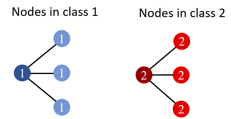
Homophily. If all edges only connect nodes with the same label, then this property is called Homophily, and the graph is call a Homophilous graph.

In Fig.1, the number denotes the label, and different colors denote distinct features. It is shown that all nodes with similar features have edges connected, and also share the same label, illustrating a perfect homophily.

Fig.1 A Homophily Example.

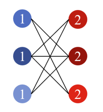
Heterophily. If all edges only connect nodes with different labels, then this kind of attribute is called Heterophily and the graph is called a Heterophilous graph. Fig.2 below shows a heterophilous graph. In this toy example, each node with label 0(1) only connects nodes with label 1(0).

Fig.2 A Heterophily Example.

Graph Homophily Ratio.

Given a graph $\mathcal{G} = {\mathcal{V, E} }$ and node label vector $y$, the edge homophily ratio is defined as the fraction of edges that connect nodes with the same labels. Formally, we have:_

\[h(\mathcal{G}, \{y_i; i \in \mathcal{V}\}) = \frac{1}{\left| \mathcal{E} \right| } \sum_{(j, k) \in \mathcal{E}} \mathbb{I}(y_j = y_k)\]

where $

\mathcal{E}

$ is the number of edges in the graph and $\mathbb{I}(\cdot)$ denotes the indicator function.

A graph is typically considered to be highly homophilous when $0.5 \le h(\cdot) \le 1$. On the other hand, a graph with a low edge homophily ratio ($0 \le h(\cdot) < 0.5$) is considered to be heterophilous.

Node Homophily Ratio.

Node homophily ratio is defined as the proportion of a node’s neighbors sharing the same label as the node. It is formally defined as:

\[h_i = \frac{1}{d_i} \sum_{j \in \mathcal{N}(i)} \mathbb{I}(y_j = y_i)\]

where $\mathcal{N} (i)$ denotes the neighbor node set of $v_i$ and $d_i = | \mathcal{N}(i) |$ is the cardinality of this set.

Similarly, node $i$ is considered to be homophilic when $h_i \ge 0.5$, and is considered heterophilic otherwise. Moreover, this ratio can be easily extended to higher-order cases $h_{i}^{(k)}$ by considering $k$-order neighbors $\mathcal{N}_k(v_i)$.

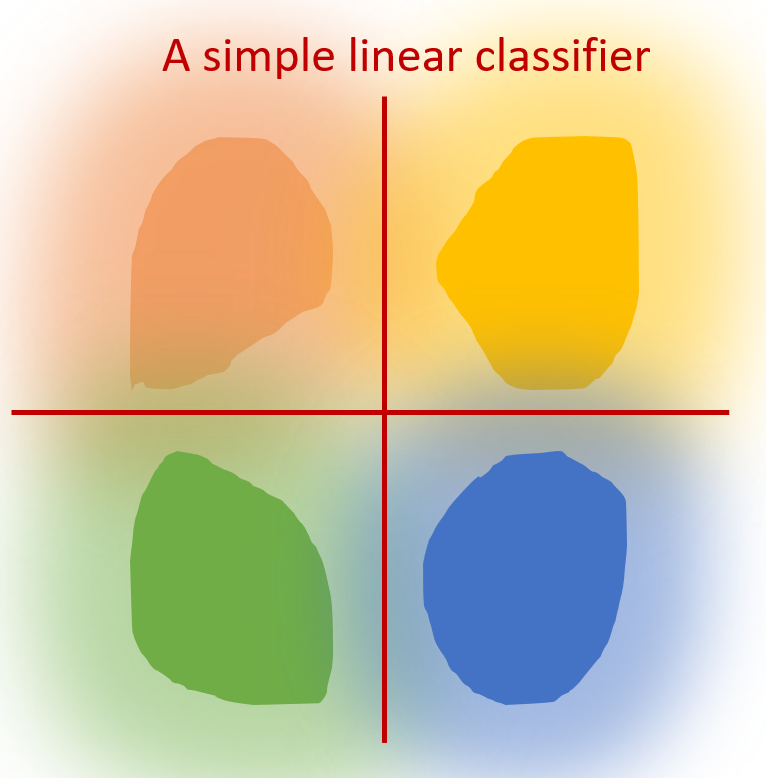
2.4 Target: What is a discriminative representation?

To examine whether GNNs perform well or not, we focus on whether GNN can encode a discriminative representatation. For instance, the ideal discrminative representation can be described as: (1) Cohension: nodes with the same label are mapped into similar representation (2) Seperation: nodes with different labels are mapped into dis-similar representations. The Fig.3 below illustrates an example of high cohension and good seperation, where each color indicates one class. We can observe that each cluster is in the same class while different clusters are distant from each other. We can then expect to use a simple linear classifier to achieve high performance, which shows an ideal representation.

Fig.3 A simple linear classifier.

3. GNN can actually do better?

In this section, we illustrate that GNNs can actually do better: Homophily, nodes connect with similar ones, which is not a necessity for the success of GNNs. GNNs can still work on various heterophily datasets (nodes connect with dissimilar ones). To achieve this goal, we focus on whether GNN can achieve discriminative representation in different settings.

3.1 Toy example & theoritical analysis

In this subsection, we examine when GCN can map nodes with the same label to similar embeddings. We first play with toy graph examples, homophily and heterophily graphs, which are shown in Section 2.3. In particular, we examine node representations from different classes after the GNN.

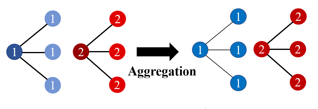
GCN under homophily: The aggregation process for the homophily graph is shown in Fig. 4, where node color and number represent node features and labels, respectively. We can easily observe that, after mean aggregation, all the nodes with class 1 are in blue, and class 2 in red, indicating a good discriminative ability. x

Fig.4 GCN under homophily.

GCN under heterophily The aggregation process for the homophily graph is shown in Fig. 5, where node color and number represent node features and labels, respectively. We can easily observe that there appears a color alternation. Before aggregation, all the nodes with class 1 are in blue, and class 2 is in red. In contrast, all the nodes with class 1 are in red, and class 2 is in blue after mean aggregation. Nonetheless, such alternation does not influence the discriminative ability. Notably, the nodes with the same class are still in the same color while nodes with different classes are in different colors, indicating a good discriminative ability.

Fig.5 GCN under heterophily.

More rigorously, we provide a theoretical understanding of what kinds of graphs could benefit from the GNNs and how. GNN can perform well on the graphs satisfying:

• Feature: Nodes from the same graph are samples from the same distribution $\mathcal{F}_{y_i}$
• Structure: Nodes from the same graph follows the same neighborhood distribution $\mathcal{D}_{y_i}$. Homophily graphs fit such an assumption, for they are more likely to be connected with nodes in the same class. Some heterophily graphs can also fit in such an assumption. For instance, Figure 5 shows that nodes in class 1 are connected with nodes in class 2 and vice versa.

The rigorous theoretical analysis are shown as follows: (You can skip the following part for heavy math!)

Consider a graph $\mathcal{G} = \mathcal{V}, \mathcal{E}, { \mathcal{F}_{c}, c \in \mathcal{C} }$, ${ \mathcal{D}_{c}, c \in \mathcal{C}} $.

For any node $i\in \mathcal{V}$, the expectation of the pre-activation output of a single GCN operation is given by \(\mathbb{E}[{\bf h}_i] = {\bf W}\left( \mathbb{E}_{c\sim \mathcal{D}_{y_i}, {\bf x}\sim \mathcal{F}_c } [{\bf x}]\right).\)

and for any $t>0$, the probability that the distance between the observation ${\bf h}_i$ and its expectation is larger than $t$ is bounded by

\[\mathbb{P}\left( \|{\bf h}_i - \mathbb{E}[{\bf h}_i]\|_2 \geq t \right) \leq 2 \cdot l\cdot \exp \left(-\frac{ deg(i) t^{2}}{ 2\rho^2({\bf W}) B^2 l}\right)\]

where $l$ denotes the feature dimensionality and $\rho({\bf W})$ denotes the largest singular value of ${\bf W}$, $B\geq\max _{i, j}|\mathbf{X}[i, j]|$.

We can than have the rigorous conclusion that the inner-class distance (distance between $h_i$ the expectation in the same class $\mathbb{E}[h_i]$) on the GCN embedding is small with a high probability, which is due to the sampling from its neighborhood distribution $\mathcal{D}_{y_i}$. Notably, the key step in the proof is the Hoeffding inequality. Details can be found in the paper.

3.2 Empirical evidence

To further verify the validity of the theoretical results, we provide more empirical evidence as follows. In particular, we manually add synthetic edges to control the homophily ratio of a graph and examine how the performance varies.

When adding synthetic heterophily edges on a homophily graph, there are two typical things to control:

• The homophily ratio: how many heterophily edges are added in a homophily graph
• The noisy ratio $\gamma$: how many edges do not follow the same neighborhood distribution $\mathcal{D}_{y_i}$. If the noisy ratio $\gamma$ is larger, the graph will be away from the condition that GNN can work well, leading to a poor performance.

As we insert heterophilous edges, the graph homophily ratio will also continuously decrease. The results are plotted in Fig.6.

Fig.6 Accuracy of GCN on the synthetic graph with various homophily ratios.

Each point on the plot in Fig.6 represents the performance of GCN model and the corresponding value in the $x$-axis denotes the homophily ratio. The point with homophily ratio $h=0.81$ denotes the original $Cora$ graph, i.e., $K=0$.

The observations are shown as follows:

• When $\gamma=0$, all edges are inserted according to the distinguished neighborhood distribution, and we observe the classification performance shows a $V$-shape pattern. This clearly demonstrates that the GCN model can work well on heterophilous graphs under certain conditions.
• When $\gamma>0$, if the noise level $\gamma$ is not so large, we can still observe the $V$-shape: e.g. $\gamma = 0.4$; this is because the designed pattern is not totally dominated by the noise. However, when $\gamma$ is larger, adding edges will constantly decrease the performance, as nodes of different classes have indistinguishably similar neighborhoods.

The experiment verifies our findings. If the neighborhood follows a similar distribution, GCN is still able to perform well under extreme heterophily. However, if we introduce noise to the neighborhood distribution, the effectiveness of GCN will not be guaranteed.

4. GNN may actually do worse

In section 3, we discuss the scenario when GNN can do well, including both homophily and heterophily graphs. All the above analyses are from a graph (global) perspective, verifying that the GNN can achieve overall performance gain. However, when we look closer into a node (local) perspective, we find the overlooked vulnerability of GNNs.

4.1 Preliminary study in node level

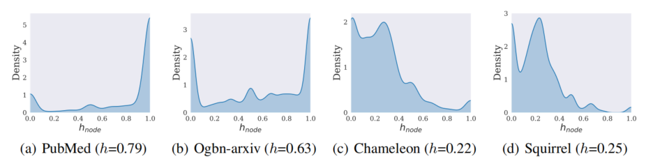
Instead of understanding from a graph perspective, the following analyses focus on nodes in the same graph but with different properties. We first plot the distribution of node homophily ratio on different datasets, shown in Fig.7. We typically include two homophily graphs and two heterophily ones. Additional results on ten different datasets can be found in the original paper. $h$ in the brackets indicating the graph homophily ratio. The $h_{node}$ on the $x$-axis denotes the node homophily ratio. We can clearly observe that:

• Regardless of global homophily and heterophily, there are both homophily nodes and heterophily nodes.
• In the homophily graph, most of the nodes are homophily nodes, where we consider the homophily patten in the homophily graph the majority pattern. Contrastively, the heterophily one will be the minor pattern.

Fig.7 Node homophily ratio distributions. All graphs exhibit a mixture of homophilic and heterophilic nodes despite various graph homophily ratios h.

Equipped with the analysis of node-level data patterns, we then investigate how GNN performs on nodes with different patterns. In particular, we compare GCN with MLP-based models since they only take the node features as the input, ignoring the structural patterns. If GCN performs worse than MLP, it indicates the vulnerability of GNNs. Experimental results are illustrated in Fig. 8.

Fig.8 Performance comparison between GCN and MLP-based models. Each bar represents the accuracy gap (MLP-based model minus GCN).

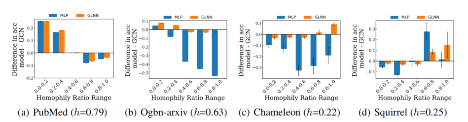
We can observe that:

• In the homophily graph, GCN works better on the homophily nodes but underperforms on the heterophily nodes.
• In the heterophily graph, GCN works better on the heterophily nodes but underperforms on the homophily nodes. Overall speaking, GNNs can work well on nodes in major pattern, but fails in minority ones. We then focus on investigating how such performance disparity happens.

4.2 Toy example & theoritical analysis

Similar to Section 3.2, we first conduct an analysis on a similar toy example. This time, instead of considering GNN under homophily and heterophily separately, we take the homophily and heterophily patterns together into consideration. The illustration is shown in Figure 9. The aggregation process for the homophily graph is shown in Fig. 4, where node color and number represent node features and labels, respectively.

Fig.9 toy example on both homophily and heterophily patterns.

We can observe that when considering the homophily and heterophily together:

• Before aggregation: nodes in class 0 are all in the blue feature, while nodes in class 1 are all in the red feature.
• After aggregation: nodes in class 0 are with both blue and red, and a similar thing in class 1. It indicates a large intra-class difference.
• After aggregation: There are some nodes with the feature blue in class 0 and some in class 1. It could be impossible to distinguish them with such small inter-class differences.

The above observations on the toy model show that GNN cannot work well on both homophily and heterophily ones. Then we further ask if GNN can learn homophily or heterophily ones well. The answer will be the majority ones in the training set.

Motivated by the toy example, we then provide theoretical understanding rigioursly from a node level. We find that two keys on test performance are:

• The aggregated feature distance between train and test nodes aggregated feature distance $\epsilon = \max_{ j \in V_m } \min_{ i \in V_{ \text{tr} } } | g_i(X, G) - g_j(X, G) |_2$ between test node subgroup $V_m$ and training nodes $V_{\text{tr}}$, where $g_i(X, G)$ is the hidden representation for node $i$.
• The homophily ratio difference $|h_\text{tr} - h_m|$.

The following theorem is based on the PAC-Bayes analysis, showing that both large aggregation distance and homophily ratio difference between train and test nodes lead to worse performance. (You can skip the following part for heavy math!)

The theory typically aims to bound the generalization gap between the expected margin loss $\mathcal{L}_{m}^{0}$ on test subgroup $V_m$ for a margin $0$ and the empirical margin loss $\hat{\mathcal{L}}_{\text{tr}}^{\gamma}$on train subgroup $V_{\text{tr}}$ for a margin $\gamma$. Those losses are generally utilized in PAC-Bayes analysis. The formulation is shown as follows:

Theorem (Subgroup Generalization Bound for GNNs):

Let $\tilde{h}$ be any classifier in the classifier family $\mathcal{H}$ with parameters ${ \tilde{W}_{l} } _{l=1}^{L}$ .

For any $0< m \le M$, $\gamma \ge 0$, and large enough number of the training nodes $N_{\text{tr}}=|V_{\text{tr}}|$, there exist $0<\alpha<\frac{1}{4}$ with probability at least $1-\delta$ over the sample of $y^{\text{tr}} = { y_i } $, $i \in V_{\text{tr}}$ we have:

\[\mathcal{L}_m^0(\tilde{h}) \le \mathcal{L}_\text{tr}^{\gamma}(\tilde{h}) + O\left( \underbrace{\frac{K\rho}{\sqrt{2\pi}\sigma} (\epsilon_m + |h_\text{tr} - h_m|\cdot \rho)}_{\textbf{(a)}} + \underbrace{\frac{b\sum_{l=1}^L\|\widetilde{W}_l\|_F^2}{(\gamma/8)^{2/L}N_\text{tr}^{\alpha}}(\epsilon_m)^{2/L}}_{\textbf{(b)}} + \mathbf{R} \right)\]

The bound is related to three terms:

(a) describes both large homophily ratio difference $|h_{\text{tr}} - h_m|$ and large aggregated feature distance $\epsilon = \max_{j\in bV_m}\min_{i\in V_{\text{tr}}} |g_i(X, G)-g_j(X, G)|_2$ between test node subgroup $V_m$ and training nodes $V_{\text{tr}}$ lead to large generalization error. $\rho= |\mu_1 - \mu_2 |$denotes the original feature separability, independent of structure. $K$ is the number of classes.

(b) further strengthens the effect of nodes with the aggregated feature distance $\epsilon$, leading to a large generalization error.

(c) $R$ is a term independent with aggregated feature distance and homophily ratio difference, depicted as $\frac{1}{N_\text{tr}^{1-2\alpha}} + \frac{1}{N_\text{tr}^{2\alpha}} \ln\frac{LC(2B_m)^{1/L}}{\gamma^{1/L}\delta}$, where $B_m= \max_{i\in V_\text{tr}\cup V_m}|g_i(X,G)|_2$ is the maximum feature norm. $\mathbf{R}$ vanishes as training size $N_0$ grows.

Our theory suggests that both homophily ratio difference and aggregated feature distance to training nodes are key factors contributing to the performance disparity. Typically, nodes with large homophily ratio differences and aggregated feature distance to training nodes lead to performance degradation.

Empirical evidence

To further verify the validity of the theoretical results, we provide more empirical evidence showing the empirical performance disparity. In particular, we compare the performance of different node subgroups divided with both homophily ratio difference and aggregated feature distance to training nodes. For a test node $i$, we measure the node disparity by

• The aggregated feature distance: selecting the closest training node $s_1 = \text{arg}\min_{v\in V_0} ||\mathbf{F}^{(2)}_u-\mathbf{F}^{(2)}_v||$.
• The homophily ratio difference $s_2 = |h^{(2)}_u - h^{(2)}_v|$.

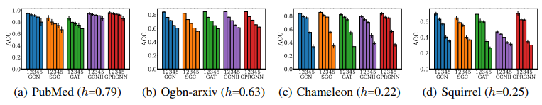
We then sort test nodes in terms of $s_1$ and $s_2$ and divide them into 5 equal-binned subgroups accordingly. We include popular GNN models including GCN, SGC (Simplified Graph Convolution), GAT (Graph Attention Network), GCNII (Graph Convolutional Networks with Inverse Inverse Propagation), and GPRGNN (Generalized PageRank Graph Neural Network). The Performance of different node subgroups is presented in Fig.9. We note a clear test accuracy degradation with respect to the increasing differences in aggregated features and homophily ratios.

Fig.9 Test accuracy disparity across node subgroups by aggregated feature distance and homophily ratio difference to training nodes. Each figure corresponds to a dataset, and each bar cluster corresponds to a GNN model. A clear performance decrease tendency can be found from subgroups 1 to 5 with increasing differences to training nodes.

We then conduct an ablation study that only considers aggregated features distance and homophily ratios in Figures 10 and 11, respectively. We can observe that the decrease tendency disappears in many datasets. Only combining these factors together provides a more comprehensive and accurate understanding of the reason for GNN performance disparity.

Fig.10 Test accuracy disparity across node subgroups by aggregated-feature distance to train nodes. A clear performance decrease tendency can be found from subgroups 1 to 5 with increasing differences to training nodes

Fig.11 Test accuracy disparity across node subgroups by homophily ratio difference to train nodes. A clear performance decrease tendency can be found from subgroups 1 to 5 with increasing differences to training nodes.

5. Applications

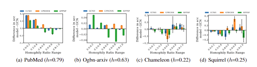
Inspired by the findings, we investigate the effectiveness of deeper GNN models on SSNC tasks.

Deeper GNNs enable each node to capture a more complex higher-order graph structure than vanilla GCN, by reducing the over-smoothing problem. Deeper GNNs empirically exhibit overall performance improvement. Nonetheless, which structural patterns deeper GNNs can exceed and the reason for their effectiveness remains unclear.

To investigate this problem, we compare vanilla GCN with different deeper GNNs, including GPRGNN, APPNP, and GCNII, on node subgroups with varying homophily ratios. Experimental results are shown in Fig.11. We can observe that deeper GNNs primarily surpass GCN on minority node subgroups with slight performance trade-offs on the majority node subgroups. We conclude that the effectiveness of deeper GNNs majorly contributes to improved discriminative ability on minority nodes.

Fig.11 Performance comparison between GCN and deeper GNNs. Each bar represents the accuracy gap on a specific node subgroup exhibiting a homophily ratio within the range specified on the x-axis.

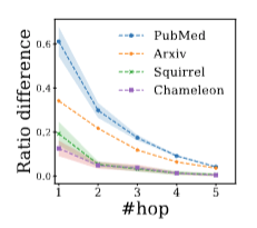
Having identified where deeper GNNs excel, reasons why effectiveness primarily appears in the minority node group remain elusive. Since the superiority of deeper GNNs stems from capturing higher-order information, we further investigate how higher-order homophily ratio differences vary on the minority nodes, denoted as, $|h_u^{(k)}-h_v^{(k)}|$, where node $u$ is the test node, node $v$ is the closest train node to test node $u$. We concentrate on analyzing these minority nodes $V_{\text{mi}}$ in terms of default one-hop homophily ratio $h_u$ and examine how $\sum_{u\in V_{\text{mi}}} |h_u^{(k)}-h_v^{(k)}|$ varies with different $k$ orders.

Experimental results are shown in Fig.12, where a decreasing trend of homophily ratio difference is observed along with more neighborhood hops. The smaller homophily ratio difference leads to smaller generalization errors with better performance.

Fig.12 Multiple hop homophily ratio differences between training and minority test nodes

6. Conclusion & suggestions & future work

In this blog, we investigate when GNN works and when not. We find that the effectiveness of vanilla GCN is not limited to the homophily graph. Nonetheless, the vulnerability is hidden under the success of GNN. We typically provide some suggestions before you build your own solution to the graph problem.

• Before starting, think carefully about your data properly
• Remember the drawback of GNNs. Not always good!

We remain some questions for future works:

• Solve the drawback of GNNs
• Inspire new principled applications on GNNs

Reference

[1]Ma, Yao and Jiliang Tang. “Deep learning on graphs.” Cambridge University Press, 2021.

[2]Ma, Yao, Xiaorui Liu, Neil Shah, and Jiliang Tang. “Is homophily a necessity for graph neural networks?.” arXiv preprint arXiv:2106.06134 (2021).

[3]Mao, Haitao, Zhikai Chen, Wei Jin, Haoyu Han, Yao Ma, Tong Zhao, Neil Shah, and Jiliang Tang. “Demystifying Structural Disparity in Graph Neural Networks: Can One Size Fit All?.” arXiv preprint arXiv:2306.01323 (2023).

[4]Kipf, Thomas N., and Max Welling. “Semi-supervised classification with graph convolutional networks.” arXiv preprint arXiv:1609.02907 (2016).

[5]Hamilton, Will, Zhitao Ying, and Jure Leskovec. “Inductive representation learning on large graphs.” Advances in neural information processing systems 30 (2017).

[6]Xu, Keyulu, Weihua Hu, Jure Leskovec, and Stefanie Jegelka. “How powerful are graph neural networks?.” arXiv preprint arXiv:1810.00826 (2018).

[7]Fan, Wenqi, Yao Ma, Qing Li, Yuan He, Eric Zhao, Jiliang Tang, and Dawei Yin. “Graph neural networks for social recommendation.” In The world wide web conference, pp. 417-426. 2019.

[8]Zhu, Jiong, Yujun Yan, Lingxiao Zhao, Mark Heimann, Leman Akoglu, and Danai Koutra. “Beyond homophily in graph neural networks: Current limitations and effective designs.” Advances in neural information processing systems 33 (2020): 7793-7804.